Process Improvement Case Study: Implementing new evaluation criteria in quality control at a TV service

One person’s measure of quality is very different from another’s. But it can create real problems in organizations when the measures of quality aren’t agreed. Here’s what happened at a major Cable TV service in Brazil, when they realized that lack of standard evaluation criteria for betacam tapes was resulting in a lot of rework and flow of materials.

The channels broadcast content that is stored on Betacam tapes and that is handled by the company’s engineering department . The original tapes are copied onto another Betacam tape, so that the original content is kept. The tape used for broadcasting is a copy that is evaluated and changed, keeping the original content intact.

The problem is that these tapes can deteriorate over time resulting in poor image quality for viewers. Or even the technical quality of the original content can be below the quality standards of the company.

The company’s engineering department was responsible for determining which tapes were fit to use for broadcast material and which weren’t. However, they had been relying upon relatively subjective measures to determine which tapes were suitable. The result was that tapes were often returned to the Channels only to find out that they had problems with them.

This meant that tapes had to be taken back to engineering resulting in rework and additional flow of material in the organization.

The organization decided to undertake a project to reduce subjectivity in this process to reduce the number of tapes returned to Channels. Several departments were involved including Processes Coordination, the Engineering Department, and Cable TV Channels.

The proposed new model

The former model of evaluation grade introduced much subjectivity in the process. The Quality Control Area classified the analysed tapes into three types: approved, approved with restrictions, condemned.

The approved with restrictions grade generated a large number of tapes returned to the Channels, increasing rework and flow of unities inside the company. Often the Channels approved the tape, due to the lack of time to ask for a replacement and due to different quality requirements between them and the Quality Control Ârea.

It was clear that the Channels requirements were different from those of QC Area. The new model would have to reduce these differences and create a common language between those involved with the process.

So, the proposed model was:

Grade = (a, b, c) where

a = number of major defects, which are perceived by the subscriber and detract from the product.

b = number of medium defects, which are perceived by the subscriber, but not enough to detract from the product.

c = number of minor defects; the subscriber does not see the problem.

This model takes into consideration the number and the intensity of defects.

This form of representation made the results more objective.

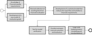
The fluxogram below shows in a high level the PDSA cycle for the project:

It was needed to plan the data collection in order to align the requirements. Before this, however, the statistical concept to be used in the new model needed to be defined.

Statistical concept used

It was necessary to work with a concept that could provide a maximum risk of returning tapes to the customers (Channels) when these tapes didn´t need to be returned. This approach would provide a reduction of the flow of materials inside the company. It would also be conservative, as a certain amount of tapes would return to the Channels, even when not necessary.

The following data was collected:

• Programme ID
• Programme Type
• Grade (ST, ME, MI), where ST = major defect, ME = medium defect, MI = minor defect
• Quality Control Evaluation
• Channel Evaluation
• Comments

This data collection plan has generated samples that has served as a basis for the application of Chebyshev´s Theorem.

For any set of data, the Russian mathematician Chebychev proved the following:

If the random variable X has a mean μ and variance σ², then for every k≥1,

P(|X−µ| ≥ kσ) ≤ 1/K²

This is the Chebyshev´s Inequality and, in words, states that:

The probability that X differs from its mean by at least k standard deviations is less than or equal to 1/k². It follows that the probability that X differs from its mean by less than k standard deviations is at least 1/k².

For a one-tailed situation, the expression is:

P(|X−µ| ≥ kσ) ≤ 1/(1+K²)

and this is the expression used in our project.

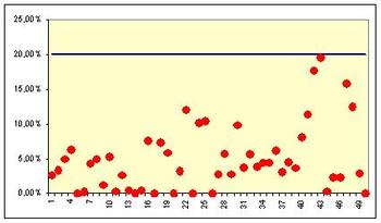
The next figure shows the results of a simulation performed by this author for 50 data sets from any type. For two standard-deviations the expression returns 20%. We can see in the figure that this limit has been respected for all the distributions. This limit will be the cutoff grade for each customer.

Practical consequence for the project:

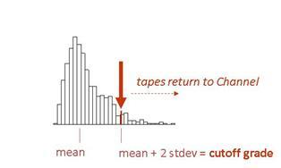
If we use a two standard-deviations limit, we will ensure that the number of tapes that return to Channel without being needed will be limited to 20%. It is a conservative model that greatly reduces the flow of tapes.

How do we apply this property to the cutoff grade of the Channels?

• The number of major, medium and light defects collected in the test spreadsheet form quantitative data sets.
• These data sets have average and standard deviation.
• We may define, for example, that the maximum probability that we accept for an occurrence of a return to a Channel of a tape that would be released is 20%.
• So, we will have the cutoff grade equal to the number of defects found for "average + two standard deviations".

It is very important to choose the correct population to be studied: Tapes that have been condemned or approved with restrictions by the Quality Control and that have been released by the Channel with no changes.

<

Collecting data

It was necessary to define a sample size for the study. A cable TV company is not used to long statistical investigations and we had to find a point between flexibility and rigor.

According to what was planned in the Plan phase we got cutoff grades for each Channel in this way:

Nearly 500 samples have been analysed in order to estimate the cutoff grades. The population has been deemed inifinite as the process is continuous and the sample size expression used was:

n= (Z*sigma/d)²

The greatest standard deviation among the standard deviations for ST, ME and MI (previous sampling) has been used, and for Z = 1.96 and d = 0.40, the sample size expression returned n = 500.

Analysing data

The cutoff grade has been estimated for the Channel that agreed to participate in the pilot test and in the next PDSA phase the results started to be compared to predictions.

It has been set up a process map for the data gathering that would confirm the success of the model implementation.

The data for this test was gathered under certain limitations, since the people from the involved areas agreed to work with only a relatively restricted sample size.

Analysis of results of cutoff grade pilot test

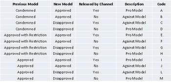
The expressions for analyzing the effectiveness of the model are going to be deduced from the various possibilities below. The model employed predicted that a maximum of 20% of tapes would return to the Channels, even when not necessary.

This model can be analysed through the expression:

(C+G)/(C+E+G)

The model approval effectiveness is analyzed trough:

(A+E+I)/(A+E+I+B+F+J)

The model disapproval effectiveness is analysed through:

(C+G+L)/(C+G+L+D+H+M)

The sample gathered resulted in:

A=0; B=0; C=3; D=10; E=93; F=3; G=24; H=9; I=0; J=0; L=0; M=0.

So,

Model ("Chebychev") effectiveness = 22.5% (n=120)

Model approval effectiveness = 96.9% (n=96)

Model disapproval effectiveness = 58.7% (n=46)

with n=sample size.

Uncertanties estimation

For the sample sizes used, the confidence intervals are:

Model ("Chebychev") effectiveness: [15.0%; 30.0%]

Model approval effectiveness: [ 93.4%; 100.0%]

Model disapproval effectiveness: [ 44.4%; 73.0%]

Understanding the results

• The model predicted a maximum of 20% of tapes would return to the Channels, even when not necessary. This value is located between the extremes of the first confidence interval (15.0% and 30.0%). Therefore we accept that the model effectiveness is confirmed by the sampling data.
• The approval effectiveness may be deemed excellent, after the confidence interval estimation. In other words, when the cutoff grade model approves a tape, the probability that the Channel also does it is very high.
• The disapproval effectiveness had the worst performance. Although the sample size results in a very large confidence interval, we can say that when the model reproves a tape, the probability that the Channel does the same is between 44.4% and 73.0%. This does not mean a great problem, because it certifies that the model is conservative (the failed tape will return to the Channel, which will decide what to do).

Benefits achieved

• New dynamics and promotion of closer relations between Channels and Quality Control.
• The synergy established has found new metrics for the evaluation process, consistent with the profile of each channel.
• Positive feedback from the representatives of the Channels.
• Reduction of internal rework, reducing costs
  Channel 1: Approximately 86% of the tapes evaluated do not return to the Channel and the quality of the product exhibited is not affected.
  Channel 2: 96%.
  Channel 3: 84%.

Analyzing the Variation at the Technical Evaluation

During the diagnostic work of the Technical Evaluation Area (Quality Control), the possibility of differences in standards of assessment among the reviewers was raised. In fact, a diagnostics of the Technical Evaluation Area became necessary and worked as a second PDSA cycle. The project team knew that, in order to achieve significant results with the use of the new cutoff grade model, it would be needed to work on a improved Technical Evaluation Area.

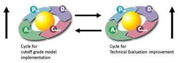
The next figure shows the relationship between the two PDSA cycles that were undertaken. This is not an usual configuration for two cycles, but it was necessary due to time constraints at that time.

Introduction

The Technical Evaluation, one of the members of the company´s Board of Engineering and Operations, represents a significant point of interaction customer/supplier or Channels/Engineering. The decisions made about changes in their process impact both the flow of tapes and the quality of what is displayed to the company´s end user. The diagnostic of the process presented here intends to identify the process critical points which will deserve improvement initiatives/redesign.

Methodology

As Is process mapping. (P)

Knowledge of the Technical Evaluation interactions with the several involved areas. (P)

Customer requirements definition. (P)

Identification of process critical factors, based on the requirements indicated and supply standards. (P)

Deployment of process failures to a level where it is possible to work effectively. (P)

Quantify factors that influence the critical process variables, when possible.(D - C)

Propose process improvements. (D - C)

Develop implementation plan for the proposed actions, together with the areas involved. (A)

Implement improvements and controls, after Engineering Management´s ok.(A)

Possible critical variables:

1 – Quality of recycled tapes.

2 – Reviewers perception of quality.

3 – IT system limitations.

4 – Channels knowledge regarding defects codes used by Technical Evaluation.

5 – Generation of a defective copy from an ok original and the sending of this copy to the Channel.

6 – Service Order filled by Internal Logistics asking the service to the Technical Evaluation.

7 – Communication among areas.

8 – Marking of blocks and time.

9 – Dissemination of standards and existing services.

10 – Requirements alignment.

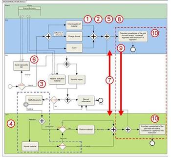
The critical variables indicated in process map were raised through process study and observation and interviews with the ones involved.

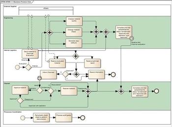
Still in the process flow diagram we can see in the right, within dotted lines, activities of filling the sheet of the pilot test of objective evaluation project, which has as one of its goals an alignment between Channels and engineering requirements. One of the deliverables of the project is to ascertain the degree of discrepancy between the requirements "supplier/customer" and elaborate the future alignment between them.

Requirements elicitation/Tree Diagram

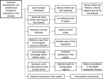
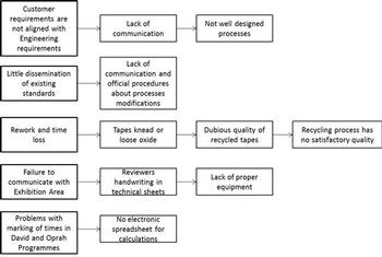
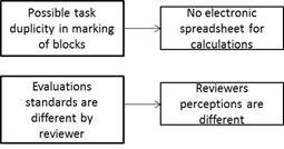
Interviews were conducted with Channels and the Internal Logistics, in search of a definition of requirements for technical evaluation. We used a tree diagram for the unfolding of the critical factors raised. Below we have the tree diagram for the variables addressed by the Technical Assessment customers. It is important to note that there is a lack of quantitative confirmation, which is not always possible.

The factors presented below (the first in the left and that are broken down into possible causes to the right) were addressed through the experience with the process by those involved.

The variables raised by the supplier (Engineering) are:

• Recycled tapes.
• Quality of the received material.
• Service Orders with filling problems.
• Delays or problems in the Media Acquisition Process.

Quantitative study of the sources of variation in the technical evaluation

One of the factors raised in the interviews with the Channels, and that could be assessed quantitatively, is the difference of perception among reviewers. This difference has an influence on the process, mainly now with the implementation of the Objective Evaluation. We know a priori that a difference of perception between humans exists, however the question that arises is whether this difference has statistical significance in the Technical Evaluation. An experiment to determine the existence of this difference in perception is the Balanced Analysis of Variance Two Factors.

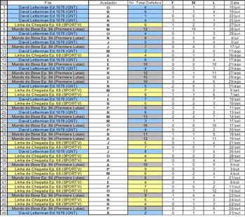
The factors to be studied are the evaluator and tape. To avoid the influence of factor equipment (which cannot be studied due to technical constraints) in the result of the experiment, we took the factor level constant, i.e., only one equipment was used. Thus, a spreadsheet for the experiment was set.

The matrix shows the combinations of randomized treatment with the factor tape having three levels (random factor) and the factor reviewer having eight levels (fixed factor). The dependent variable registered is the total number of defects, which is subdivided into major, medium and minor.

Obs.: "Fita" = "Tape" / "Avaliador" = "Reviewer" / "Nr. Total Defeitos" = "Total Number of Defects" / "F" = "MA" / "M" = "ME" / "L" = "MI".

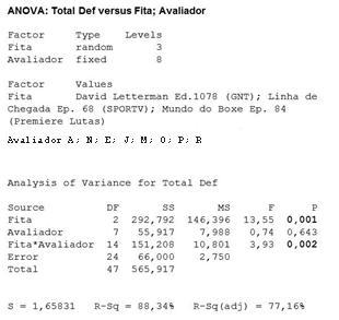
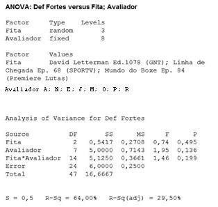
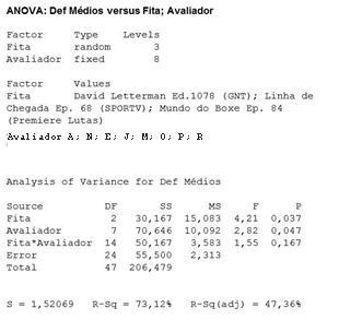
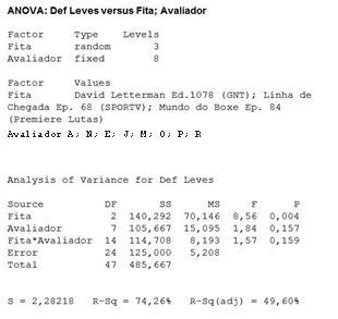
Minitab outputs are shown below:

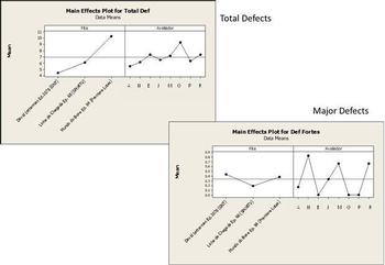
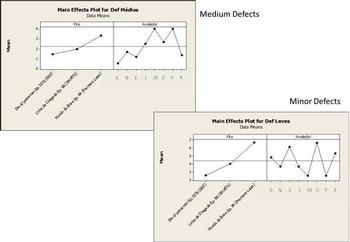
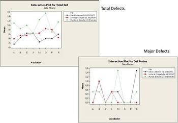
• Thus, considering the response variable Total Defects, the significant effects are Tape (main effect) and Tape*Evaluator (interaction effect). That is, the tape that is being evaluated is a significant influence on the total number of defects. And it depends on the evaluator that is evaluating.
• For the response variable Major Defects, it is seen that no effect is statistically significant. This is somewhat understandable, since major defects present less difficulty for the evaluator.
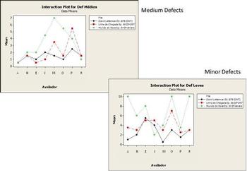
• For Medium Defects, we have two statistically significant effects, Tape and Evaluator. It is due to the difficulty in defining what is "medium".
• For Minor Defects, Tape is a significant factor (main effect). That is, a change in the response (number of minor defects) is statistically significant when changing the tape that is being evaluated.

The Tape is the factor that most influences the response of the average defect count (ST, ME and MI). One might expect such a result, since there are different programs for the different channels. We also must pay attention to the fact that the factor Evaluator influences the Medium Defects count.

Medium defects remain a challenge to the perception of the evaluators, being difficult to classify (it seems). The interaction of the evaluator with the tape, influencing the total defects, should also be considered carefully, because the evaluator´s performance may depend on the tape that is being evaluated, resulting in increased variation in the assessment process and inconsistency of results.

Below we find the main and interaction effects plots and we can see that they reflect what ANOVA p-values estimate.

Quantitative study of the quality of recycled tapes

The quality of recycled tapes and their performance during the technical evaluation appear frequently among the variables raised by the Channel and Engineering as responsible for possible problems during the process. Thus, a quantitative test was planned and executed under the leadership of the ??Processes Coordination.

We can say that the percentage of recycled tapes that have trouble and are condemned in the Technical Evaluation (major drop out, kneading and drop oxide) is between 1.65% and 7.45%.

Action Plan

The main variable identified was the discrepancy between the quality requirements between Engineering and the Channel, and it has already been addressed by the Project "Objective Grade", which is meeting the expectations of the project team and clients of Technical Evaluation. The alignment of the quality requirements between supplier and customers will benefit process control, Engineering and Channels. It will decrease rework, limiting the number of tapes that return unnecessarily to the Channel after evaluation and creating a less subjective language to communicate the quality of the tapes. It is recommended to the reader to be acquainted with the project mentioned.

Other significant variables have been identified:

- Difference in evaluation standards by an reviewer (detailed in "Quantitative study of the sources of variation in the Technical Evaluation").

- Communication problems between suppliers and customers.

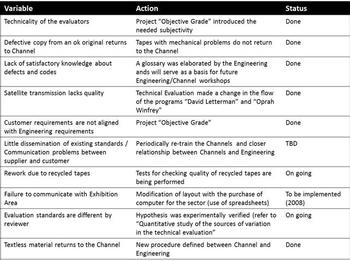
The following table shows the actions implemented / in progress / to be implemented to improve the technical evaluation by the time of project implementation.

A training, aiming to reduce the difference between the perceptions of the evaluators, has been provided. A reviewer was chosen as standard and the tape used by Engineering ("defects examples") will be redone based on his perception. Other evaluators will be trained with this new tape, and the glossary of defects may need to receive some modification. The rating of the difference of perception between observers will become regular, and it is expected that this difference reaches the goal set by the management area, as the training occurs. Nowadays (2013) there is a periodic workshop on the subject.

A Clients Handbook has been developed, including a glossary of defects.

The model continues to be applicable, even with the evolution of technology, where we went from a SD standard to a HD standard and from manipulation of tapes to manipulation of content.

Considerations from the statistical and methodological viewpoints

• The most important assumption used in the project was that the grades data sets mantained their shapes approximately the same, in order that the cutoff grades estimated by Chebyshev´s Innequality would not change significantly. This would correspond to a reasonable degree of statistical control along the months. Of course, it is not easy to achieve, mainly because this implies a homogeneity of data which is not typical of these kind of processes. However, as the results have indicated, the model is enough robust so that it can work in the real world.
• Due to the difficulties usually encountered in the company for running tests with significant sample sizes, the uncertanties are traditionally large. However, they provide a reasonable basis for decision. So far, the cutoff grade model appears to be efective.
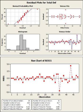
• The check of residuals from the Balanced Analysis of Variance Two Factors indicates that they have mean equal to zero but are not normally distributed (maybe a little departure from normality). When they are plotted on a Run Chart, we don´t find evidences of non-randomness. Regarding an eventual non-normality of residuals, it has already been demonstrated that Analysis of Variance is a robust procedure. Usually, if the residuals look odd, something strange may be happening. The original observations may not be independent, or the variables have markedly different variance. Non-normality of the original observations may have an effect, but as Box (1953) stated, this is generally not a problem:

So far as comparative tests on means are concerned it appears (perhaps rather surprisingly) that this practice is largely justifiable, for thanks to the work of Pearson (1931), Bartlett (1935), Geary (1947), Gayen (1950 a, b), David & Johnson (1951 a, b) there is abundant evidence that these comparative tests on means are remarkably insensitive to general non-normality" of the parent population.

• The two PDSA cycles were undertaken practically at the same time. We might say that a better configuration would be run firstly the PDSA cycle for the Technical Evaluation improvement, because the variation reduction in the area would contribute positively for the conclusions from the cutoff grade model implementation. Schedule restrictions, however, obliged the project team to work simultaneously in both cycles.